Hypothesis Testing with BPP
Getting Started
Download one of the archives that have the data and pre-configured control files for today’s exercises here.
Introduction
There are now a range of tools for detecting historical gene flow between species or populations from genomic data. This might involve searches with network models, tests with site patterns, or other lines of evidence. The goal of this exercise is to understand how full-likelihood methods can be a tool for testing multiple competing hypotheses and divergence time estimation to help us bridge the gap between patterns and processes. There are other full likelihood implementations of multispecies network coalescent or related models, but we will focus on the BPP software.
Our test data is a small sample of North American dry ferns (Dryopteris). These are interesting because a lot is known about relationships between diploid progenitors and the allopolyploids. Can we get the relationship between diploids and an allotetraploid correct? We have a reduced set of 30 loci from a target enrichment experiment. The relationships among all Dryopteris are a bit complex , but we simplify the story by using a small sample and limiting ourselves to a level-1 network.
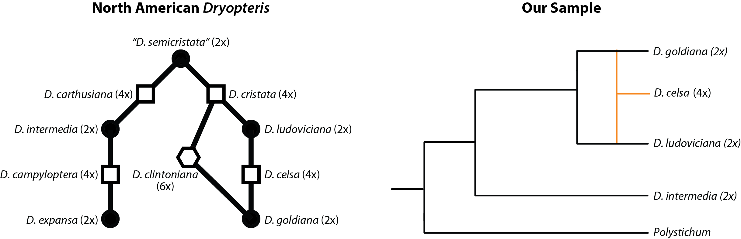
Adapted from Fig. 1 of Tiley et al. 20211- Relationships between North American Dryopteris and their ploidy levels. Our example data includes one allotetraploid.
Full-likelihood methods provide us a powerful tool because we can evaluate multiple competing hypotheses in a statistically sound probabilistic framework. However, it can be tempting to compare as many competing models as possible. In practice, this will be difficult due to computational burdens or our inability to explain the rational for every possible model. A successful application of BPP or similar full-likelihood programs relies on your knowledge of the system and their natural history, and perhaps prior analyses with a range of phylogenetic or population genetic tools. Our network hypothesis here is bolstered by a long history of chromosome investigations and previous phylogenetic results with a few Sanger loci.
How to specify a network
Formatting networks correctly can be difficult, especially when we want to specify the direction of gene flow. Luckily, BPP comes with a simple program to help create network models based on simpler binary trees. Consider our backbone topology - we will add some node labels for our convenience too. We can create a simple text file msci-create.in that provides the backbone topology as well as the branch that gene flow goes from and the branch that gene flow goes into. Multiple gene flow events can be specified here and the branch lengths of the introgression edges can be constrained if appropriate:
tree (Pmun,(Dint,(Dlud,(Dcel,Dgol)u)t)s)r;
hybridization t Dlud, u Dcel as i j tau=yes, yes phi=0.2
Here, we have allowed the divergence time of the introgression edges from their parental lineages to be different from the age of introgression. We specify an initial introgression probability of 0.2. The introgression probability will be sampled by the MCMC algorithm, so this is only a starting value. We can generate the network used for our analyses with the following command:
bpp --msci-create msci-create.in > msci-create.out
Below is the resulting network that we can add to our control file. You should try to draw the network yourself from the text string and convince yourself this is correct.
(Pmun, (Dint,((j[&phi=0.200000,tau-parent=yes],Dlud)i,((Dcel)j[&phi=0.800000,tau-parent=yes],Dgol)u)t)s)r;
The BPP control file
All aspects of data input, results output, and the model specification are done within the control file. An example looks like this:
          seed =  219527

       seqfile = Dryopteris.bppDat
      Imapfile = Dryopteris.spmap
       outfile = 4.1.out
      mcmcfile = 4.1.mcmc

  speciesdelimitation = 0
         speciestree = 0

   speciesmodelprior = 1  * 0: uniform LH; 1:uniform rooted trees; 2: uniformSLH; 3: uniformSRooted

  species&tree = 5  Pmun Dint Dgol Dcel Dlud
                    1 1 1 1 1
		    (Pmun, (Dint,((j[&phi=0.200000,tau-parent=yes],Dlud)i,((Dcel)j[&phi=0.800000,tau-parent=yes],Dgol)u)t)s)r;
      phase = 0 0 0 0 0

      usedata = 1  * 0: no data (prior); 1:seq like
      nloci = 30  * number of data sets in seqfile

      cleandata = 0    * remove sites with ambiguity data (1:yes, 0:no)?

      thetaprior = 2 0.01 e  # invgamma(a, b) for theta
      tauprior = 3 0.02    # invgamma(a, b) for root tau & Dirichlet(a) for other tau's
      clock = 1
      model = hky
      alphaprior = 2.4 4 4
   phiprior = 1 1
      locusrate = 1 0 0 10 iid

      finetune =  1: 0.3 0.3 0.01 0.05 0.3 0.3 1.0 0.3
         print = 1 0 0 0   * MCMC samples, locusrate, heredityscalars, Genetrees
        burnin = 20000
      sampfreq = 10
      nsample = 10000
      threads = 4 1 1
All of the options and parameters are explained very well in the BPP manual, but here is a short explanation:
- seed = random number used to generate starting conditions for the MCMC algorithm
- seqfile = input sequences. BPP uses a phylip format with all loci in one file
- Imapfile = a text file matching individuals to their species. You can sample multiple individuals per species under the MSC
- outfile = the primary output of BPP with parameter estimates
- mcmcfile = the log file of all mcmc samples
- Setting speciesdelimitation and speciestree to 0 instruct BPP to estimate parameters on a fixed topology. We are not searching for the network.
- The species&tree option specifies
- The number of species in the tree
- Those species names in the tree that must match the Imapfile
- The number of individuals per species
- The network hypothesis (potentially generated from msci-create)
- phase = Are sequences haploid or diploid (Ambuguity codes represent heterozygosity)
- usedata = Keep as 1 to use the sequence data. Sometimes, it can be helpful to run the MCMC algorithm without data (option 0) to investigate the marginal priors and if your data have information
- nloci = the number of loci
- Theta varies across nodes, but the same prior is used on all thetas (the expected number of nucleotide differences per site between two sequences sampled from the population). BPP uses an inverse gamma distribution that has a long tail for the MCMC to explore higher values if need be. A distribution mean on 0.01 is probably fine for species.
- The Tau prior uses an inverse gamma on the root and the other nodes are a little more complicated. Making sure the prior is difuse and then inspecting that the posterior pulls away from the prior is probably reasonable enough.
- clock = 1 means all branches have the same rate of evolution (a strict clock). There are options for relaxing these assumptions but a strict clock is reasonable for closely related species without major life history variation.
- The prior on the introgression probability is a beta distribution. Using the parameters her turns that beta into a uniform distribution.
- print = BPP can give you a lot of information, but here we keep it simple and keep only the mcmc output
- burnin = the number of samples to skip as burnin. This does NOT account for the sample frequency
- sampfreq = the number of samples to skip before saving one after the burnin is complete
- nsample = the total number of posterior samples to save from the analysis
- threads = BPP can be faster by distributing loci among different threads. Here, we can assume everyone has at least 4 available
Parameter estimation and convergence
We can run BPP using our example control file and data. Change into the BPP-Workshop folder and you will find the sequence data Dryopteris.bppDat and the individual-to-species map Dryopteris.spmap. Have a look to get a feel for the formatting. If you prepare the individual-to-species map file for your own data, the input data for BPP can be prepared by the formatBPPdata.pl script from a collection of aligned fasta files in the exampleData_30loci folder.
Change into Converge and then the folder for model 4 4 and run BPP on one of the prepared control files by:
cd Converge
cd 4
bpp --cfile 4.1.ctl
The MCMC analysis will start. It will take a while even for our small dataset. While that is running, we can look at some finished runs and evaluate convergence and look at the results. I have already completed 4 runs for all models with the same MCMC settings. A popular tool for analyzing convergence is Tracer. It is a useful tool, but I am a big believer that chasing ESS scores might not be the best for complex introgression models. Instead, we will run an R script to summarize some information for us, and if we are satisfied, we can use BPP to use all of our MCMC samples for parameter estimation.
cd ../../Converge-completed/4
R CMD BATCH plotPosteriors.R
Alternatively, you can run the R script from Rstudio or the R shell. A quick check of all of the parameter posteriors is that they look pretty similar. I think a good indication of convergence is a comparison of the median node heights (divergence times). If everything went well, our estimates should be very close to a one-to-one relationship.
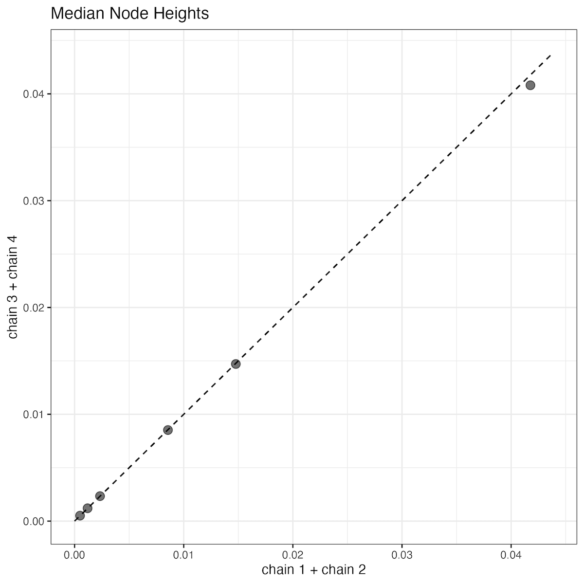
Median node heights from four MCMC runs- The posteriors from runs 1 and 2 or 3 and 4 are combined to display in the scatter plot. The dotted line is the one-to-one line.
In my opinion, everything looks good! We could benefit from a larger sample frequency and probably an increased burnin here, but it is acceptable. For reporting our results, there are two choices:
- Report the results of the first MCMC analysis, since everything converged
- Combine the MCMC sample across runs, if we need to increase our sample size
You are fine doing either but depending on your reviewer, they might tell you to do the other. If you want to generate the BPP output for the combined sample, we can concatenate the MCMC output from the 4 runs together, but there is only 1 header line. This was done for
combined.mcmc. Then we need to make a new control filecombined.ctlwith some edits:
          seed =  219527

       seqfile = ../../Dryopteris.bppDat
      Imapfile = ../../Dryopteris.spmap
       outfile = combined.out
      mcmcfile = combined.mcmc

  speciesdelimitation = 0
         speciestree = 0

   speciesmodelprior = 1  * 0: uniform LH; 1:uniform rooted trees; 2: uniformSLH; 3: uniformSRooted

  species&tree = 5  Pmun Dint Dgol Dcel Dlud
                    1 1 1 1 1
		    (Pmun, (Dint,((j[&phi=0.200000,tau-parent=yes],Dlud)i,((Dcel)j[&phi=0.800000,tau-parent=yes],Dgol)u)t)s)r;
      phase = 0 0 0 0 0

      usedata = 1  * 0: no data (prior); 1:seq like
      nloci = 30  * number of data sets in seqfile

      cleandata = 0    * remove sites with ambiguity data (1:yes, 0:no)?

      thetaprior = 2 0.01 e  # invgamma(a, b) for theta
      tauprior = 3 0.02    # invgamma(a, b) for root tau & Dirichlet(a) for other tau's
      clock = 1
      model = hky
      alphaprior = 2.4 4 4
   phiprior = 1 1
      locusrate = 1 0 0 10 iid

      finetune =  1: 0.3 0.3 0.01 0.05 0.3 0.3 1.0 0.3
         print = -1 0 0 0   * Changing print to -1 will only summarize the mcmcfile
        burnin = 20000
      sampfreq = 10
      nsample = 40000
*      threads = 4 1 1
Notice the the mcmcfile is now our combined sample as input. We then change print to -1 and this will instruct BPP to bypass the MCMC and summarize the mcmcfile as the new outfile. If you every want to comment out a line in the control file, you can uses a “*”, like I did for the threads option.
Can you find the mean age of introgression for our allotetraploid and its 95% highest posterior density (HPD) interval in the output file? How does your new run compare when it is finished? You can add the results of your new run to a google sheet.
What if we do not have a model that we trust, but have multiple competing hypotheses? The next steps will show us techniques for comparing models, but I recommend some analysis like above across some or all of your hypotheses to check that your MCMC settings are sufficient. What can happen is that as model complexity increases (i.e. more introgression edges), you will need longer sample intervals and longer burn-ins. Settings that work well for a binary tree might be problematic for networks and this should be checked in advance before you realize the problem after computationally intense analyses.
Marginal likelihoods and model probabilities
Likelihood methods are great because they often allow us to compare and rank models. But a complication of Bayesian methods is that we have a sample of likelihoods rather than a single maximum likelihood estimate. Additionally, Bayesian estimators will be influenced by the prior distributions we imposed. There has been rigorous investigation into methods for estimating the marginal likehood where those confounding effects of the prior are factored out. The stepping-stone method Xie et al. 20112 has had good performance in a range of other phylogenetic applications and we will use it again here. BPP can generate samples of the power posteriors (Rannala and Yang 20173) that we can use to calculate the marginal likelihoods and model probabilities either from the bppr R package or by hand. We will compare 7 models today:
| Model | Description |
|---|---|
| 1 | D. celsa sister to D. ludoviciana |
| 2 | D. celsa sister to D. goldiana |
| 3 | D. goldiana sister to D. ludoviciana |
| 4 | D. goldiana and D. ludoviciana are progenitors of D. celsa |
| 5 | D. goldiana and D. ludoviciana are progenitors of D. celsa |
| 6 | D. goldiana and D. ludoviciana are progenitors of D. celsa |
| 7 | Model 4 with introgression from D. ludoviciana into D. goldiana |
Marginal likelihoods are time-intensive, because the require us to generate an MCMC sample for multiple values of beta, the factor that allows us to integrate out the prior. We do not have time to cover the details of why, but let’s get started doing and there is room for discussion after.
To estimate the marginal likelihood we need to generate the series of power posteriors. A reasonable number of steps can be hard to determine, but you can repeat the analysis for an increasing number of steps to check stability of the marginal lnL estimate. I tend to use 24 steps for my work. We will use 8 here to speed up the process.
Some files have been prepared for you. Go ahead and start your first run for your assigned model. For example, if you have model 1, do:
cd YOUR_PATH/BotanyWorkshop/BF-8/1/1
bpp --cfile 1.1.bf.ctl
When it is done, complete the other 7 runs. These will go fast because I have made the MCMC very short…too short. But while you wait, there is a question about setting up the analysis. The only difference in these control files versus out previous ones is that the line BayesFactorBeta = 1e-300 was added to the bottom of 1.1.bf.ctl. By the 8th run, this says BayesFactorBeta = 5.129089e-01. My preference is to let the bppr R package generate these values for my, but BPP also comes with an option called bfdriver or you can calculate them yourself. With the bppr, I generated the values for the number of points by
make.beta(8,method="step-stones",a=5)
You could then generate the necessary control files and folder structure and a file of the beta values called beta.txt with:
make.bfctlf(b, ctlf="controlfile.ctl", betaf="beta.txt")
but because I find myself working on shared university clusters, especially to distribute the jobs over many processors. You will notice a prepared control file that has all of the models included and they are commented out. I use the Perl script genBFctl.pl to use the template.ctl and beta.txt file to generate all of the necessary control files on the cluster. You can use that or bppr if more comfortable, but you will need to prepare a control file for each model.
Once all of the runs are done for the 8 steps. You can calculate the marginal likelihood. In R, go to the directory with the 8 folders for your model. For example model 1:
library(bppr)
setwd("YOUR_PATH/BPP-Workshop/BF-8/1")
my.model <- stepping.stones(mcmcf="mcmc.txt",betaf="../beta.txt")
This works because the mcmc output from each run is called mcmc.txt. Have a look at the object created called my.model. Can you find the marginal lnL and the standard error? Add those to the google sheet. We can do the model probability calculations by hand, but you can use the predone runs in BF-8-completed to generate the model probabilities and their 95% confidence intervals based on a bootstrap from bppr. For example:
setwd("YOUR_PATH/BotanyWorkshop/BF-8-completed/1")
model.1 <- stepping.stones(mcmcf="mcmc.txt",betaf="../beta.txt")
setwd("../2")
model.2 <- stepping.stones(mcmcf="mcmc.txt",betaf="../beta.txt")
setwd("../3")
model.3 <- stepping.stones(mcmcf="mcmc.txt",betaf="../beta.txt")
setwd("../4")
model.4 <- stepping.stones(mcmcf="mcmc.txt",betaf="../beta.txt")
setwd("../5")
model.5 <- stepping.stones(mcmcf="mcmc.txt",betaf="../beta.txt")
setwd("../6")
model.6 <- stepping.stones(mcmcf="mcmc.txt",betaf="../beta.txt")
setwd("../7")
model.7 <- stepping.stones(mcmcf="mcmc.txt",betaf="../beta.txt")
bayes.factors(model.1,model.2,model.3,model.4,model.5,model.6,model.7)
These are from longer MCMC runs. How do the results compare to our short runs? Model 4 is the least worst, but do you feel comfortable rejecting our more complex model 7? You can see results from more steps and more loci on sheet 3 of the google sheet.
Bayes factor approximation with the Savage-Dickey density ratio
Despite the rigor and computation of Bayes factors, there is some concern for preferring unnecessarily more complex models, or perhaps your error yields confidence intervals on the model probabilities that yields the interpretation ambiguous (Tiley et al. 20234). Another tool is available to us that requires a fraction of the computing - an approximation of the Bayes factor for nested models using the Savage-Dickey density ratio (Ji et al. 20235). We can approximate the Bayes factor of model 7 versus model 4 because 7 adds only one more introgression edge. In R, we
setwd("YOUR_PATH/BPP-Workshop/Converge-completed/7")
model.7.mcmc <- read.table(file="7.1.mcmc",header=TRUE,sep="\t")
# The epsilon values from Tiley et al. (2023) were 0.01 and 0.001.
cutoff <- 0.01
# The number of posterior samples where the introgression probability from D. ludoviciana to D. goldiana is less than cutoff
nlowphi <- 0
for (i in 1:length(model.7.mcmc$phi_l..k))
{
	if (model.7.mcmc$phi_l..k[i] < cutoff)
	{
		nlowphi <- nlowphi + 1
	}
}
# The posterior probability that the introgression probability of interest is less than our negligible region
posterior.probability <- nlowphi/length(model.7.mcmc$phi_l..k)
# The Savage-Dickey Ratio approximation of the Bayes factor for model7/model4
sd.bayes.factor <- cutoff/posterior.probability
We can consult the tables of Kass and Raftery (1995)6 to interpret our Bayes factor result. Note this is not on any log scale. I calculated 0.04014452, which means we can reject the 2-rate model, and this happens to be about the 3% significance level. Try repeating the calculation with a smaller cutoff of 0.001 to ensure stability of our results. Thus, the Savage-Dickey ratio approximation can be an good strategy if your models are nested and you can generate good posteriors of the phi values.
Limits to Biological Interpretations
In our Dryopteris test case, we are lucky such that the biology is already worked out over years of meticulous chromosome work combined with multiple molecular studies. Unknown systems do not have this advantage and the lifetime of an investigation may not be long enough for long-term experimental work. It can be tempting to use network methods to infer the process of hybridization or polyploidization, but I strongly caution against this. Processes other than hybrid speciation can explain high introgression probabilities (Tiley et al. 20234) and inferring extant parental species can be dubious if there are sampling gaps among species. But we have seen in this limited example that full-likelihood methods perform well at characterizing the relationship of our Dryopteris species even if the model is probably much simpler (i.e. a single episodic origin) than the truth. The parameter estimates might be interesting, but we can also calculate probabilities for competing models. Luckily, our approaches do not seem to only favor complexity. If the model probabilities are too close for comfort and if your hypotheses are well constrained, approximation of the Bayes factor with the Savage-Dickey density ratio is simple and might be helpful for us to sort out technical artifacts of other analyses versus biologically meaningful information.
References
-
Tiley GP, Crowl AA, Manos PS, Sessa EB, Solís-Lemus C, Yoder AD, Burleigh JG. 2021. Phasing alleles improves network inference with allopolyploids. bioRxiv doi: https://doi.org/10.1101/2021.05.04.442457
↩ -
Xie W, Lewis PO, Fan Y, Kuo L, Chen M-H. 2011. Improving marginal likelihood estimation for Bayesian phylogenetic model selection. Syst Biol 60:150-160
↩ -
Rannala B, Yang Z. 2017. Efficient Bayesian species tree inference under the multispecies coalescent. Syst Biol 66:823-842
↩ -
Tiley GP, Flouri T, Jiao X, Poelstra JW, Xu B, Zhu T, Rannala B, Yoder AD, Yang Z. 2023. Estimation of species divergence times in presence of cross-species gene flow. Syst Biol doi: https://doi.org/10.1093/sysbio/syad015
↩ ↩2 -
Ji J, Jackson, D, Leaché AD, Yang Z. 2023. Power of Bayesian and Heuristic Tests to Detect Cross-Species Introgression with Reference to Gene Flow in the Tamias quadrivittatus Group of North American Chipmunks. Syst Biol 72:446-465
↩ -
Kass RE, Raftery AE. 1995. [Bayes factors.] Journal of the American Statistical Association 90:773-795. - Access through JSTOR or some of the free pdfs floating about online.
↩